Stochastic Gradient Descent (SGD)

pseudocode:

# true sgd (batch size is 1)
for sample in dataset:
	g = compute_gradient(sample, θ)
	θ = θ - a * g

# mini-batch sgd (batch size is 32, 256, ... 512 for gpt2, 3.2M for gpt3)
for batch in dataset:
	g = compute_gradient(batch, θ)
	θ = θ - a * g

I prove that stochastic gradient descent convergences to a loss of zero given some initial assumptions here. (If the vanilla SGD convergence proof already looks like that, I'm glad this field is empirical! I now understand why in his 2010 paper on GLU variants, Shazeer writes that "we offer no explanation as to why these architectures seem to work; we attribute their success, as all else, to divine benevolence.")

The overall motivation for the optimizers below is that we can update different parameters differently, with the cost of extra memory, and this can lead to better performance.

Momentum (Polyak, 1964)

Momentum adds a velocity term that accumulates gradients over time - prevents getting stuck in local minima.

v = zeros_like(θ)   # velocity value for each parameter

for batch in data:
    g = compute_gradient(batch, θ)
    v = β * v + (1 - β) * g    # moving average
    θ = θ - a * v

Nesterov Momentum (1983) evaluates the gradient at the future point, after the momentum is applied.

v = zeros_like(θ)   # velocity value for each parameter

for batch in data:
    v_prev = v
	g = compute_gradient(batch, θ)
	v = β * v - a * g 
	θ = θ - β * v_prev + (1 + β) * v

RMSProp (Hinton, 2012)

RMSProp normalizes each parameter's update by its typical gradient magnitude. For example: if gradient 1 is 0.001 and gradient 2 is 100, a fixed learning rate would not be work well. This fixes the exploding and vanishing gradient problems.

s = zeros_like(θ)  # squared gradient average for each parameter

for batch in data:
    g = compute_gradient(batch, θ)
    s = β * s + (1 - β) * g²    # moving average
    θ = θ - a * g / (√s + ε)    # normalize by RMS, ε to avoid division by 0

Adam (Kingma and Ba, 2014)

Adam is Momentum + RMSProp with bias correction for better moving averages near the start of training.

m = zeros_like(θ)  # momentum for each parameter
s = zeros_like(θ)  # squared gradient avg for each parameter

for batch in data:
    g = compute_gradient(batch, θ)
	m = β₁ * m + (1 - β₁) * g      # first moment (momentum)
	v = β₂ * v + (1 - β₂) * g²     # second moment (RMSProp)
	m̂ = m / (1 - β₁ᵗ)              # bias correction
	v̂ = v / (1 - β₂ᵗ)              # bias correction
	θ = θ - a * m̂ / (√v̂ + ε)

The team introduced another variant of Adam with weight decay, a regularization technique that penalizes large parameter values.

m = zeros_like(θ)  # momentum for each parameter
s = zeros_like(θ)  # squared gradient avg for each parameter

for batch in data:
    g = compute_gradient(batch, θ)
	m = β₁ * m + (1 - β₁) * (g + λ * θ)      # first moment (momentum) + weight decay
	v = β₂ * v + (1 - β₂ * (g + λ * θ)²     # second moment (RMSProp) + weight decay
	m̂ = m / (1 - β₁ᵗ)              # bias correction
	v̂ = v / (1 - β₂ᵗ)              # bias correction
	θ = θ - a * m̂ / (√v̂ + ε)

AdamW (Loshchilov and Hutter, 2017)

Idea: weight decay should shrink parameters uniformly, not be subject to the adaptive learning rates. We apply the weight decay separately.

m = zeros_like(θ)  # momentum for each parameter
s = zeros_like(θ)  # squared gradient avg for each parameter

for batch in data:
    g = compute_gradient(batch, θ)
	m = β₁ * m + (1 - β₁) * g             # first moment (momentum) 
	v = β₂ * v + (1 - β₂) * g²            # second moment (RMSProp)
	m̂ = m / (1 - β₁ᵗ)                     # bias correction
	v̂ = v / (1 - β₂ᵗ)                     # bias correction
	θ = θ - a * m̂ / (√v̂ + ε) - a * λ * θ  # weight decay

Muon (Jordan et al., 2024)

Idea: instead of adapting the learning rate per parameter using second moments (squared gradient avg), we adapt the update direction by orthogonalizing the momentum matrix. This helps because in practice, the momentum matrix becomes domindated by a few directions (some rows have much greater momentums than others), and orthogonalization creates a new direction that explores dimensions equally.

We can only apply Muon to 2D parameters, like linear layers, attention weights (Q, K, V projections), MLP weights, and hidden layer weights. The remaining weights, like biases, use AdamW.

Notice that this uses half the memory that AdamW uses.

m = zeros_like(θ)  # momentum for each parameter

for batch in data:
    g = compute_gradient(batch, θ)
    m = β * m + (1 - β) * g                    # momentum
    m̂ = orthogonalize_if_matrix(m)             # orthogonalize 2D params only
    ŝ = compute_scale_if_matrix(g, m̂)          # scale to match gradient magnitude
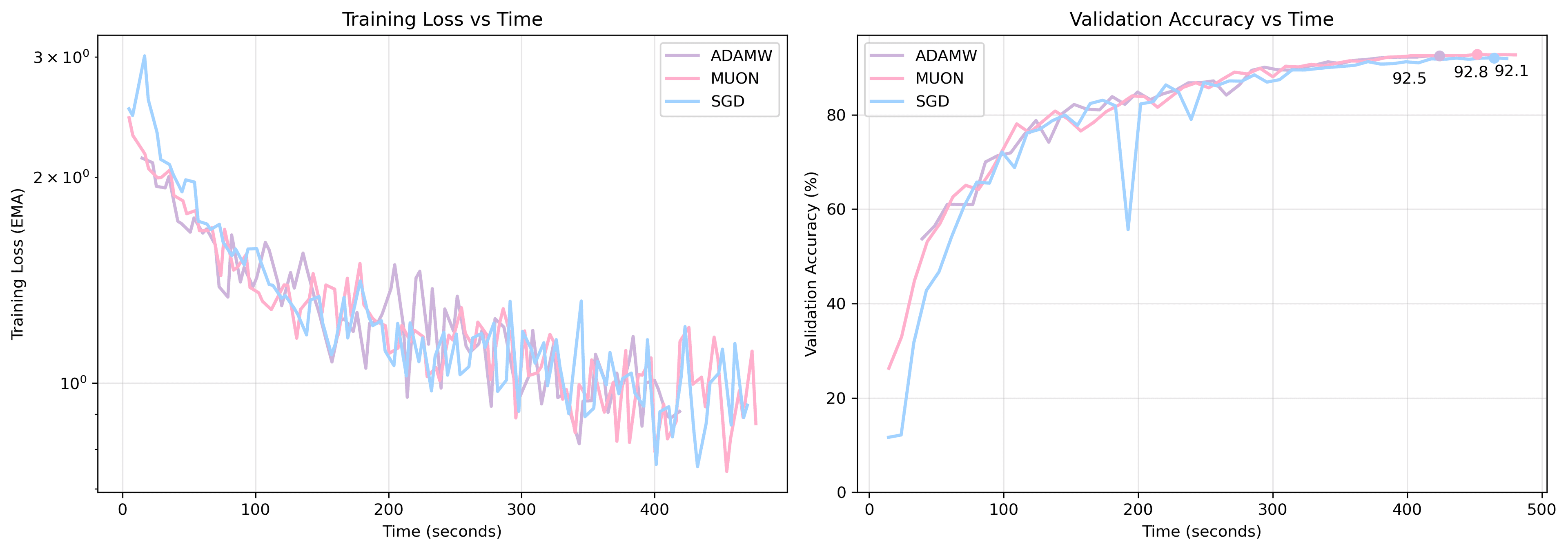
    θ = θ - a * ŝ * m̂ - a * λ * θ              # update with weight decay

Optimizer Comparisons

Below is a comparison of SGD (with Nesterov momentum), AdamW, and Muon on ResNet-50 with CIFAR-10. The difference between Muon and AdamW here are marginal, possibly because ResNet-50 is relatively small and Muon can shine where there are larger 2D weight matrices.

Next steps: (1) look at the math behind Muon. particularly, what does it mean when the Kimi team writes that "Muon offers a norm constraint that lies in a static range of Schatten-p norm" in the 'Muon is Scalable' paper? (2) compare these optimizers on more complex tasks (ImageNet) and larger models (LLMs). If you want to sponsor some compute for these experiments, reach out!